
BallEngine

Attractor 3D:
Chaos with a recognisable shape

Tens of thousands of particles tracing a chaotic equation that never retraces its path and never leaves its own bounded silhouette.
Play the preview

In development0 creators want this next

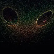
A frame from Attractor 3D
Open the studio to run this mode live.

Attractor 3D is being built right now

The engine, the physics and the look are done enough to watch. What is not finished is everything around them: the settings, the presets and the export path. So we shipped it as a preview instead of sitting on it.

The order is decided by these votes rather than by us, and the most-voted modes go first. If this is the one you want, say so.

What you can do now
Open it in the studio and watch a full run, with sound, exactly as it stands today.
What is held back
Settings, randomize and export. The preview runs on our defaults so every viewer judges the same version.
When it ships
The most-voted unfinished mode is the one we take next.

What Attractor 3D does

Tens of thousands of GPU particles tracing a strange attractor: a cloud that never repeats itself and never leaves its own silhouette.

A strange attractor is the solution set of a chaotic differential equation. Follow it and you never retrace your path, never settle into a cycle, and never leave a bounded region. The result is a shape that is simultaneously always changing and always recognisable, which is a rare and useful property for a visual.

Attractor 3D traces one with tens of thousands of particles integrated in a fragment shader. The cloud endlessly reshapes itself while holding a silhouette you could pick out of a lineup: the Lorenz butterfly, the Rössler spiral, and dozens of others besides.

Each equation is data rather than code. Forty-eight coefficients over a monomial basis, plus a measured profile giving its world scale, framing offset, integration rate and safe timestep. That is what lets the catalogue be large without every entry needing its own hand-tuned camera.

How a run plays out

The exact sequence the engine runs in this mode, from the first frame to the moment the run resolves.
  1. 1.

    An equation is chosen

    Each attractor is forty-eight coefficients over a monomial basis, together with a measured profile for scale, framing, integration rate and safe timestep.

  2. 2.

    Particles integrate on the GPU

    Tens of thousands of particles advance through the equation in a fragment shader, which is what makes a cloud of that size possible at full frame rate.

  3. 3.

    The silhouette holds

    Because the trajectory never leaves the attractor’s bounded region, the cloud keeps its recognisable overall shape no matter how long it runs.

  4. 4.

    The beat can morph it

    Morph On Beat switches equation on a musical cue, so the cloud reorganises into a different attractor in time with the track.

Every control in Attractor 3D

These are the settings this mode adds on top of the shared physics, visual, audio, and export controls. Names match the studio sidebar exactly.

Attractor

  • Attractor
  • Equation

The equation is the subject of the video. Some are wide and flat, some are dense and vertical, and the framing profile is measured per equation so each one is presented properly.

Particles

  • Particles
  • Particle Count

Count is the density of the trace. Low counts read as a sketch of the shape, high counts as a solid volume with internal structure.

Look

  • Look
  • Colour By
  • Ramp Start
  • Ramp End

Colouring by velocity or by position reveals the internal structure of the attractor, which a single flat colour hides completely.

Caption and beat

  • Equation Caption
  • Show The Equation
  • Caption Text
  • Alignment
  • Text Color
  • Beat Response
  • Morph On Beat
  • Own Sounds
  • Morph Sound

Showing the equation is a genuine hook for this audience. It tells the viewer that the shape is a consequence of three lines of maths.

Why Attractor 3D videos hold attention

What keeps people watching this mechanic.

It never repeats

There is no loop point to notice, so the video does not develop the staleness that most generative visuals acquire after ten seconds.

The silhouette is memorable

A recognisable overall shape gives the eye something stable to hold while the detail keeps changing.

The equation caption is a hook

Showing that this comes from three lines of maths converts a pretty visual into something people want to explain to someone else.

Morphs punctuate the run

Changing equation on the beat gives an otherwise continuous visual a set of discrete events to structure it.

Videos you can make in this mode

Each of these is a different configuration of the same mode, so one setup session produces a batch of related uploads.

Single attractor

One equation held for the whole run with the caption shown. The clearest presentation.

Morph sequence

Equations switching on the beat so the cloud reorganises repeatedly. More structured and more musical.

Velocity-coloured

Colour by speed so the fast and slow regions of the attractor separate visually.

Dense volume

A high particle count so the attractor reads as a solid object with internal layers.

Sparse sketch

A low count so individual trajectories are followable, which shows what the equation is actually doing.

Equation series

One video per attractor from the catalogue, each captioned. A large series from one setup.

Make your first Attractor 3D video

The order that works. Following it out of sequence usually means retuning settings you already set.
  1. 1.

    Pick the equation

    Browse the catalogue and choose a silhouette. The framing profile is measured per equation, so it will present correctly.

  2. 2.

    Set the particle count

    Higher for a solid volume, lower for a legible sketch. This is the single biggest look decision after the equation.

  3. 3.

    Colour by motion

    Colour by velocity or position so the internal structure is visible rather than hidden inside a flat mass.

  4. 4.

    Show the equation

    Turn the caption on. It is what tells the viewer this is maths rather than an effect.

  5. 5.

    Add beat morphs

    If the run is long, morph on the beat so it has structure rather than being one continuous state.

Settings that make the difference

  1. Show the equation. This is one of the few visuals where explaining it makes it more impressive.
  2. Colour by velocity is almost always better than a flat colour, because it reveals where the trajectory speeds up.
  3. A lower particle count is not a compromise. Sparse traces show what the equation does; dense ones show what it looks like.
  4. Morphing on the beat is the cheapest structure available for a visual with no natural events.
  5. The equations are data, so trying a different one costs one setting rather than a rebuild.

What breaks a run

  1. A flat single colour at a high particle count, which produces an undifferentiated blob.
  2. Morphing too often, so no attractor is on screen long enough to be recognised.
  3. Hiding the caption, which throws away the strongest hook this mode has.
  4. Choosing a wide flat attractor for a vertical canvas without checking the framing.

Never repeating, never leaving

The property that makes a strange attractor useful here is a pair of opposites held at once. The trajectory is chaotic, so it never retraces itself and never falls into a cycle. It is also bounded, so it never wanders off and never grows without limit.

For a video that means the detail is always new while the overall shape is always the same. A viewer gets both the stability that lets them recognise what they are looking at and the novelty that stops them feeling they have seen it.

Most generative visuals fail one of those tests. Loops repeat and become stale; unbounded systems drift out of frame or collapse. This is a category of system that structurally does neither, which is why it is worth the shader work.
Equations as data

Each attractor here is forty-eight coefficients over a monomial basis. That representation is general enough to cover the classical named systems and a large number of others, and it means adding an attractor is adding a row rather than writing code.

The harder part is presentation. A raw equation says nothing about how large its attractor is, where its centre sits, how fast to integrate it, or what timestep stays stable. Those four numbers are measured per equation and stored alongside the coefficients.

Without that profile, a catalogue of this size would be unusable: every entry would need its camera framed by hand, and a viewer switching equations would get a cloud too small to see or one clipping out of frame. With it, switching attractor is a single setting that always presents correctly.

Attractor 3D questions

Open Attractor 3D

Every control on this page is already in the studio. Load the mode and start from a working run.